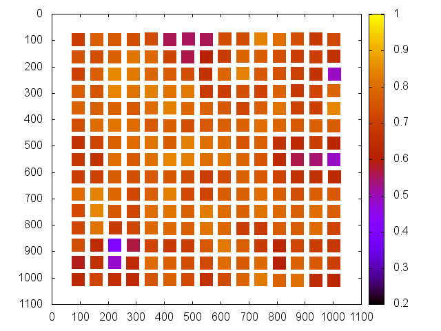
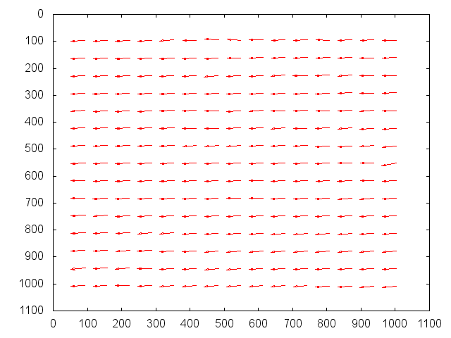
|
Size: 4190
Comment:
|
Size: 6282
Comment:
|
| Deletions are marked like this. | Additions are marked like this. |
| Line 5: | Line 5: |
| The results show no significant difference in the final CompareOBJ RMS regardless of how poor the viewing conditions are, however a visual inspection of the topography clearly shows the degradation and poor representation that occurs as imaging conditions become qualitatively "worse". As a proxy for accuracy, we can instead | The results show no significant difference in the final CompareOBJ RMS regardless of how poor the viewing conditions are, however a visual inspection of the topography clearly shows the degradation and poor representation that occurs as imaging conditions become qualitatively "worse". As a proxy for accuracy, we can instead look at statistics based on a normalized cross correlation between the generated topography and truth topography. The results of comparing both the target area as a whole, and the individual high resolution maplets to the truth topography more clearly demonstrates the relationship between the quality of observing conditions and the quality of the topography. |
| Line 7: | Line 7: |
| It should be noted that S/C position perturbation was divided equally between the SCOBJ components, resulting in a distance from the truth position which was a multiple of the standard deviation of 6.4m. Therefore: * maximum lateral perturbation was a multiple of 3.7m (6.4m/sqrt(3)); * normal perturbation (wrt body center) was 3.7m (6.4m/sqrt(3)). It is assumed that the worst case scenario is a 3 x sigma (19.2m) lateral perturbation. The maximum possible lateral perturbation tested was 3 x 3.7m = 11.1m. |
|
| Line 12: | Line 8: |
| In all cases, the final SPC-derived S/C position is within 8m of the true S/C position, but in only two cases is within 2m of the true S/C position. The actual distance from the true S/C position is not dependent on the initial perturbed position - for example in the 0.25 x sigma case, the SPC-derived S/C position (distance from truth: 1.6m to 6.9m) in most cases moves further away from the true S/C position than its initial position (distance from truth: 1.6m). The final SPC-derived S/C positions appear to be clustered around an incorrect solution 2m-8m distant from the true S/C position. |
It should also be noted that while the cross correlation values have a maximum of 1, comparing two samplings of the truth topography to one another generates a value of 0.833. This is a reasonable result for reasons which are not discussed here, but this is purely to give a metric by which to compare values. |
| Line 18: | Line 12: |
| CompareOBJ does not appear to be affected by the magnitude of S/C position and pointing perturbation within the ranges tested. | CompareOBJ does not appear to be affected largely by the quality of imaging conditions. We have come to realize that RMS is not a sufficient means of evaluating topography for accuracy in and of itself, but rather should be used in addition to other criteria. |
| Line 20: | Line 14: |
| {{attachment:CompareOBJ_RMS_resized.png}} | |
| Line 22: | Line 15: |
| '''CompareOBJ Optimal Translations:''' ||'''Sub-Test'''||'''Perturbation Magnitude'''||||||'''Translation (cm)'''|| ||F3G7||0.25 x sigma||85.0698||62.3596||-14.3765|| ||F3G6||0.50 x sigma||84.5538||61.6624||-15.3434|| ||F3G5||0.75 x sigma||95.8438||59.9313||-21.6901|| ||F3G3||1.00 x sigma||106.4870||58.2162||-27.3527|| ||F3G4||1.50 x sigma||79.1224||63.2865||-19.6432|| ||F3G2||2.00 x sigma||110.1339||58.9454||-23.2403|| ||F3G1||3.00 x sigma||93.5937||61.6997||-26.8422|| |
'''CompareOBJ RMS:''' ||'''Sub-Test'''||'''RMS (cm)'''||'''Optimal Trans-Rot RMS (cm)'''||'''Kabuki RMS (cm)'''|| ||F3C1||N/A||N/A||N/A|| ||F3C2||65.999||16.116||9.886|| ||F3C3||54.171||20.513||11.075|| ||F3C4||63.450||21.909||10.617|| ||F3C5||64.596||16.583||9.905|| ||F3C6||66.583||16.845||9.253|| There are a few caveats to the above results that are important to understand. First, we now know that there is a shift of approximately 2m of the coordinate system between the truth model and the evaluation model. This does not have an effect on the topography, just its location in 3D space. This means that the plain CompareOBJ RMS is fundamentally calculating RMS in the wrong place, and thus the values in the second column of the above table are fairly meaningless. Next, it is also known that CompareOBJ's translation and rotation optimization algorithm does not always find the correct location, which is indeed what is happening here. We have used other tools (primarily Meshlab) to verify that these translations are indeed incorrect. This means that the RMS values in the third column above, while closer to the truth than those in column two, are still incorrect. The values in the final column are the most meaningful RMS values we have as we used a hand calculated initial guess for the necessary translation, and then optimized RMS around that location. It can be seen then that there is no large deviation in RMS between the subtests, but the values in general do increase with degrading imaging conditions. F3C3 was expected to have the worst conditions and had the worst RMS; while F3C6 had the best imaging conditions and had the best RMS. |
| Line 34: | Line 31: |
| The first graph shows footprints for all Detailed Survey PolyCam pictures which were included in the model. The second graph shows the four pictures down-selected due to their coverage of the 20m x 20m evaluation region, and their almost complete containment within the iterated 100m x 100m region. | These figures show the image footprints on the surface for each subtest. The bold lines outline the 50x50 m study region. Some images overlap almost exactly, so the total number of images is written along with the figure. |
| Line 36: | Line 33: |
| {{attachment:vertices_all_resized.png}} | {{attachment:F3C1imgPrint.png}} |
| Line 38: | Line 35: |
| {{attachment:vertices_eval_resized.png}} | Images: 4 |
| Line 40: | Line 37: |
| == Distance SCOBJ(truth) to SCOBJ(solution) == | |
| Line 42: | Line 38: |
| The distance of the final SPC-derived S/C position from the true S/C position is plotted for the full Detailed Survey PolyCam image set for each magnitude of perturbation. The evaluation images are plotted in red. | {{attachment:F3C2imgPrint.png}} |
| Line 44: | Line 40: |
| 3D graphs of final SPC-derived SCOBJ and true SCOBJ are then plotted for each picture. The first four are the down-selected evaluation pictures, the rest of the image set is included for comparison. | Images: 4 |
| Line 46: | Line 42: |
| The pattern of final SPC-derived SCOBJ is broadly consistent across magnitudes of perturbation. The position correction is mostly a normal correction with lateral movement, bringing the modeled S/C position within an approx. 8m-radius sphere around the true position (or, in the case of perturbations<8m, pushing SCOBJ outwards up to 8m). | |
| Line 48: | Line 43: |
| {{attachment:scobj_distance_resized.png}} | {{attachment:F3C3imgPrint.png}} |
| Line 50: | Line 45: |
| === Evaluation Pictures === | Images: 3 |
| Line 52: | Line 47: |
| '''Example nominal SCOBJs:''' | |
| Line 54: | Line 48: |
| {{attachment:P601293751G3_nominal_resized.png}} | {{attachment:F3C4imgPrint.png}} |
| Line 56: | Line 50: |
| ''' Final solution SCOBJs:''' | Images: 3 |
| Line 58: | Line 52: |
| {{attachment:P601293751G3_final_resized.png}} | |
| Line 60: | Line 53: |
| {{attachment:P601372862G2_final_resized.png}} | {{attachment:F3C5imgPrint.png}} |
| Line 62: | Line 55: |
| {{attachment:P601372868G2_final_resized.png}} | Images: 8 |
| Line 64: | Line 57: |
| {{attachment:P601372874G2_final_resized.png}} | |
| Line 66: | Line 58: |
| === Remaining Detailed Survey PolyCam Pictures === | {{attachment:F3C6imgPrint.png}} |
| Line 68: | Line 60: |
| {{attachment:P601293196G2_final_resized.png}} | Images: 8 |
| Line 70: | Line 62: |
| {{attachment:P601293757G3_final_resized.png}} | |
| Line 72: | Line 63: |
| {{attachment:P601372298G3_final_resized.png}} | |
| Line 74: | Line 64: |
| {{attachment:P601372304G3_final_resized.png}} | == Normalized Cross Correlation == |
| Line 76: | Line 66: |
| {{attachment:P601372310G3_final_resized.png}} | A normalized cross correlation (NCC) analysis was done both on the evaluation bigmap (20x20 m) as a whole, and the individual 5 cm/pixel maplets that form the 50x50 m study region. The outputs of the NCC analysis on the full bigmaps are pictured below with their respective correlation values. Visually it is easy to see from the figure in the upper right hand corner of each plot that the topography is drastically affected by the imaging conditions. Features on the surface move about, and the bigmap clarity is worse for poorer viewing conditions. |
| Line 78: | Line 68: |
| {{attachment:P601372316G3_final_resized.png}} | <<BR>> === F3C2 === {{attachment:C2.png}} <<BR>>Correlation Score: 0.6940 |
| Line 80: | Line 73: |
| {{attachment:P601372856G2_final_resized.png}} | <<BR>> === F3C3 === {{attachment:C3.png}} Correlation Score: 0.6238 === F3C4 === {{attachment:C4.png}} Correlation Score: 0.5996 === F3C5 === {{attachment:C5.png}} Correlation Score: 0.6664 === F3C6 === {{attachment:C6.png}} Correlation Score: 0.7650 Next the statistics for each maplet in the 50x50 m study region are below. The correlation value was plotted for each maplet in terms of x-y position on the truth bigmap to show where the topography performs better or worse. In addition, the individual translations are plotted to show the distance each maplet had to move to where the correlation was found. Seeing strong agreement in the translations is very encouraging because we know we have a bias error of approximately 2m in our model. From these translations we are able to come up with exclusion criteria for maplets which correlated in an incorrect location. We set a standing 100 pixel translation for a fail criteria, and a 5 pixel deviation from average as a marginal boundary. This is useful because while a maplet may have a high correlation, if it is in the wrong place, this correlation is meaningless. The statistics for each subtest are outlined in the table below, and all values were calculated after the outliers (moved more than 100 pixels) were removed from the set. ||'''Sub-Test'''||'''Average Translation (px)'''||'''Standard Deviation (px)'''||'''Pass/Marg/Fail (%)'''|| ||F3C2||39.658||0.903||96.82/0.00/3.18|| ||F3C3||40.099||0.906||88.00/2.22/9.78|| ||F3C4||37.627||1.902||82.19/5.02/12.79|| ||F3C5||41.820||1.074||97.78/0.89/1.33|| ||F3C6||41.179||0.600||99.11/0.89/0.00|| '''F3C2''' {{attachment:F3C2cor.png}} {{attachment:F3C2trans.png}} '''F3C3''' {{attachment:F3C3cor.png}} {{attachment:F3C3trans.png}} '''F3C4''' {{attachment:F3C4cor.png}} {{attachment:F3C4trans.png}} '''F3C5''' {{attachment:F3C5cor.png}} {{attachment:F3C5trans.png}} '''F3C6''' {{attachment:F3C6cor.png}} {{attachment:F3C6trans.png}} |
TestF3G - Results
Comments
The results show no significant difference in the final CompareOBJ RMS regardless of how poor the viewing conditions are, however a visual inspection of the topography clearly shows the degradation and poor representation that occurs as imaging conditions become qualitatively "worse". As a proxy for accuracy, we can instead look at statistics based on a normalized cross correlation between the generated topography and truth topography. The results of comparing both the target area as a whole, and the individual high resolution maplets to the truth topography more clearly demonstrates the relationship between the quality of observing conditions and the quality of the topography.
It should also be noted that while the cross correlation values have a maximum of 1, comparing two samplings of the truth topography to one another generates a value of 0.833. This is a reasonable result for reasons which are not discussed here, but this is purely to give a metric by which to compare values.
CompareOBJ RMS
CompareOBJ does not appear to be affected largely by the quality of imaging conditions. We have come to realize that RMS is not a sufficient means of evaluating topography for accuracy in and of itself, but rather should be used in addition to other criteria.
CompareOBJ RMS:
Sub-Test |
RMS (cm) |
Optimal Trans-Rot RMS (cm) |
Kabuki RMS (cm) |
N/A |
N/A |
N/A |
|
65.999 |
16.116 |
9.886 |
|
54.171 |
20.513 |
11.075 |
|
63.450 |
21.909 |
10.617 |
|
64.596 |
16.583 |
9.905 |
|
66.583 |
16.845 |
9.253 |
There are a few caveats to the above results that are important to understand. First, we now know that there is a shift of approximately 2m of the coordinate system between the truth model and the evaluation model. This does not have an effect on the topography, just its location in 3D space. This means that the plain CompareOBJ RMS is fundamentally calculating RMS in the wrong place, and thus the values in the second column of the above table are fairly meaningless. Next, it is also known that CompareOBJ's translation and rotation optimization algorithm does not always find the correct location, which is indeed what is happening here. We have used other tools (primarily Meshlab) to verify that these translations are indeed incorrect. This means that the RMS values in the third column above, while closer to the truth than those in column two, are still incorrect.
The values in the final column are the most meaningful RMS values we have as we used a hand calculated initial guess for the necessary translation, and then optimized RMS around that location. It can be seen then that there is no large deviation in RMS between the subtests, but the values in general do increase with degrading imaging conditions. F3C3 was expected to have the worst conditions and had the worst RMS; while F3C6 had the best imaging conditions and had the best RMS.
Image Footprints
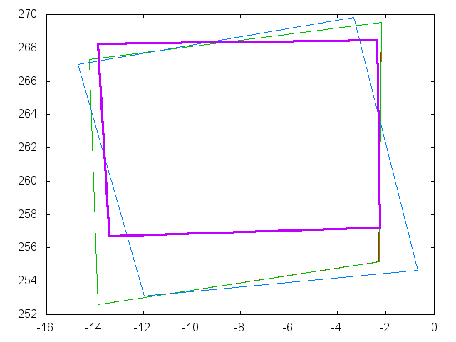
These figures show the image footprints on the surface for each subtest. The bold lines outline the 50x50 m study region. Some images overlap almost exactly, so the total number of images is written along with the figure.
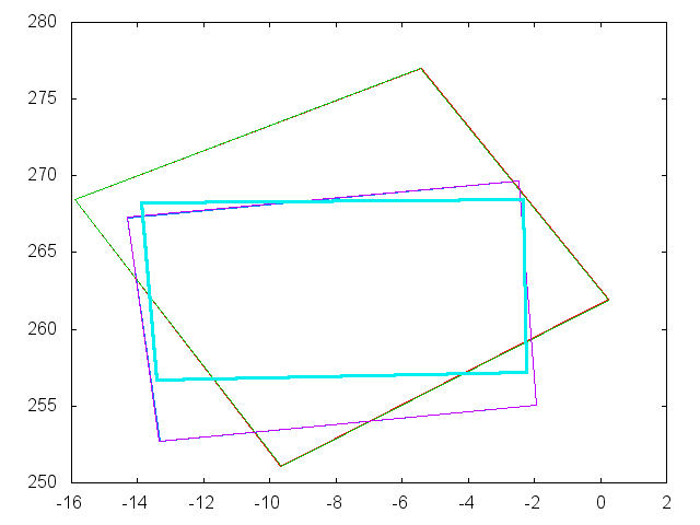
Images: 4
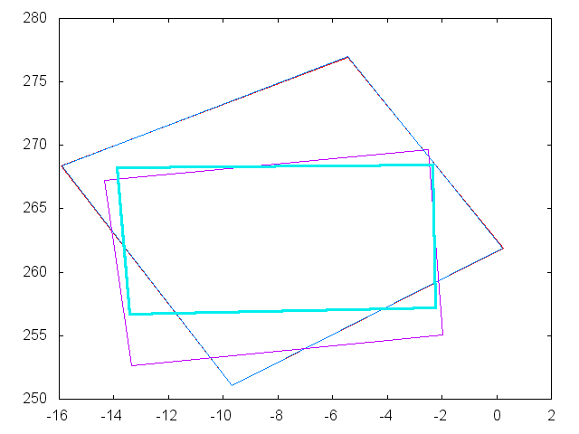
Images: 4
Images: 3
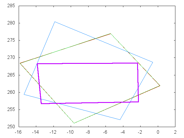
Images: 3

Images: 8
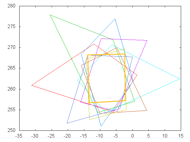
Images: 8
Normalized Cross Correlation
A normalized cross correlation (NCC) analysis was done both on the evaluation bigmap (20x20 m) as a whole, and the individual 5 cm/pixel maplets that form the 50x50 m study region. The outputs of the NCC analysis on the full bigmaps are pictured below with their respective correlation values. Visually it is easy to see from the figure in the upper right hand corner of each plot that the topography is drastically affected by the imaging conditions. Features on the surface move about, and the bigmap clarity is worse for poorer viewing conditions.
F3C2

Correlation Score: 0.6940
F3C3

Correlation Score: 0.6238
F3C4

Correlation Score: 0.5996
F3C5

Correlation Score: 0.6664
F3C6
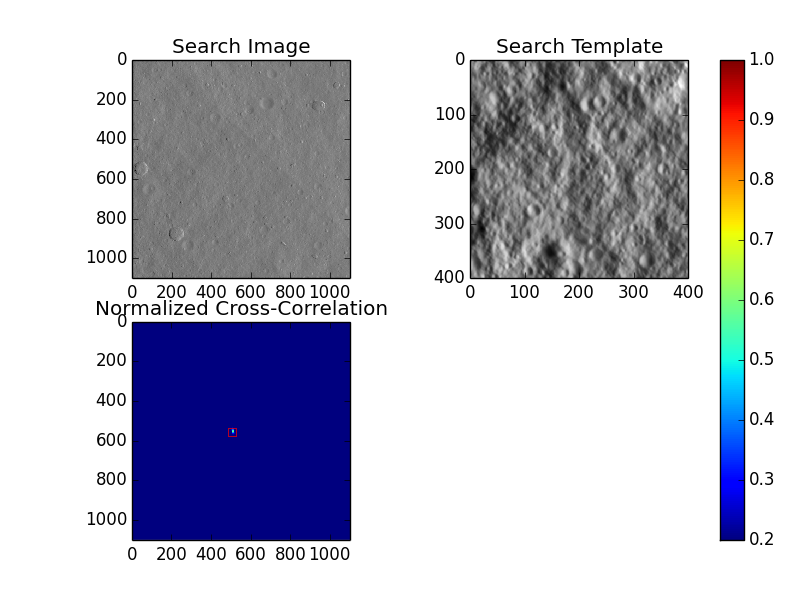
Correlation Score: 0.7650
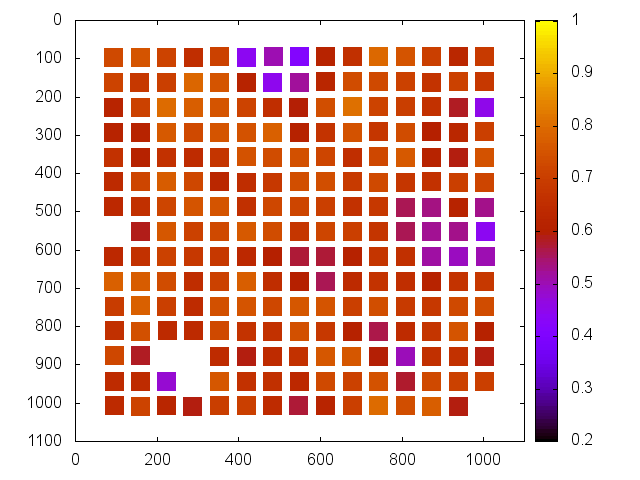
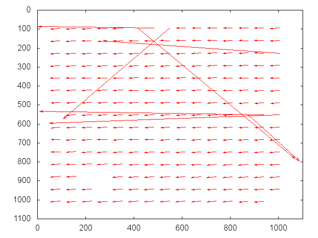
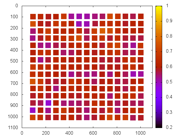
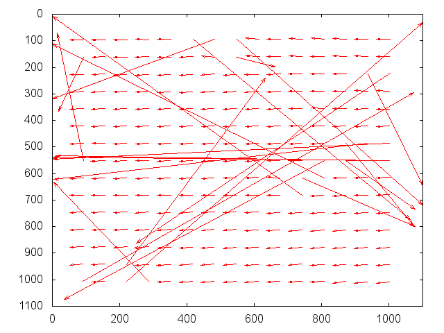
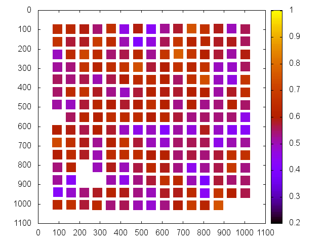
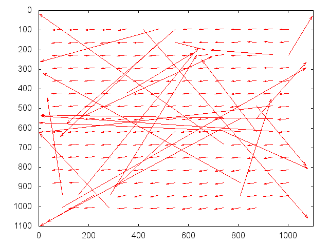
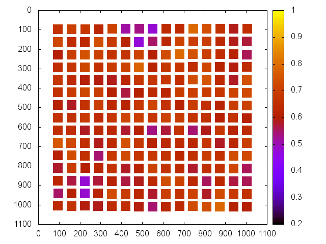
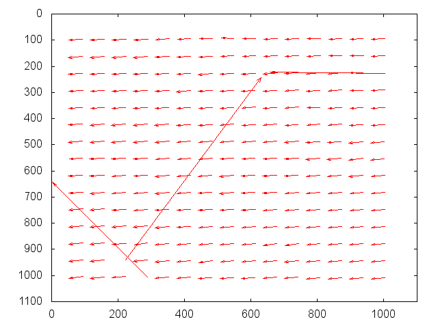
Next the statistics for each maplet in the 50x50 m study region are below. The correlation value was plotted for each maplet in terms of x-y position on the truth bigmap to show where the topography performs better or worse. In addition, the individual translations are plotted to show the distance each maplet had to move to where the correlation was found. Seeing strong agreement in the translations is very encouraging because we know we have a bias error of approximately 2m in our model. From these translations we are able to come up with exclusion criteria for maplets which correlated in an incorrect location. We set a standing 100 pixel translation for a fail criteria, and a 5 pixel deviation from average as a marginal boundary. This is useful because while a maplet may have a high correlation, if it is in the wrong place, this correlation is meaningless. The statistics for each subtest are outlined in the table below, and all values were calculated after the outliers (moved more than 100 pixels) were removed from the set.
Sub-Test |
Average Translation (px) |
Standard Deviation (px) |
Pass/Marg/Fail (%) |
39.658 |
0.903 |
96.82/0.00/3.18 |
|
40.099 |
0.906 |
88.00/2.22/9.78 |
|
37.627 |
1.902 |
82.19/5.02/12.79 |
|
41.820 |
1.074 |
97.78/0.89/1.33 |
|
41.179 |
0.600 |
99.11/0.89/0.00 |
